


A dynamic macroeconomic model
My personal tool for macroeconomic forecasting, v1.0

In this post I present a rather technical working tool for macroeconomic forecasting, my very own workhorse strutural model. This model is an ongoing project, subject to constant development. I expect to adjust this technical note whenever I find use for an update.
The model is structural as it is comprised of endogenous variables whose interactions allow for a degree of self-determination across them, based on initial conditions provided by data. It is dynamic, capturing all the expected transition phases until variables reach a steady state. Its purpose is to allow for economic theory-consistent forecasting, scenario analysis, stress-testing and informed storytelling. This is all achieved by stating a system of differential equations. Lets get to it.
Section 1: The endogenous core system
The following equations will be the core part of our model, laying out the dynamics of our endogenous variables.
Equation 1, the Investment-Savings (IS) curve:
Where ‘y’ stands for the output gap, a measure of economic spare capacity, or, in other words, the distance between effective demand and the long run supply of goods (potential output). Meanwhile, “Et[y(t+1)]” is an expression for the expectation of the output gap one period ahead, “i” is a reference for the market interest rate, “Et[π(t+1)]” represents the expectation for the one period ahead inflation rate (denoted as “π”), “i[bar]” stands for the long run neutral interest rate and “π[bar]” the central bank inflation target, “ε(y)” represents a stochastic shock, assumed to follow a normal distribution “N(μ,σ)” with “μ=0” and constant “σ”.
Throughout the description of our equations, you’ll notice a couple of “β’s”, these are linear parameters (we'll swap those for time-fixed numbers later on).
This equation is known as a linearized Euler equation, derived from a standard intertemporal consumption problem often found is New Keynesian DSGE models.
Equation 2, a hybrid Phillips curve (PC):
Here, we introduce variables “π[imp]” and “ε(π)”, representing what we call imported inflation (the variation on a commodity price index "𝜅” multipled by the nominal exchange rate minus expected inflation) and a cost-push stochastic inflationary shock, also assumed normally distributed and uncorrelated with our previous demand shock “ε(y)”.
The Phillips curve captures the inflation dynamics of an economy. In this setting, we allow for an economy compromised with backward and forward looking firms, that is, firms that reset prices based on past “π(t-1)”, and expected “Et[π(t+1)]” inflation. Theoretical justifications for this equation are found in standard firm profit maximization problems, where price setters (firms) seek to adjust prices toward margins over real marginal costs (often approximated by output gaps), also common in DSGE models.
However, it is important to notice that the imported inflation component “π[imp]” is rather an augmentation of our hybrid Phillips curve, more commonly found in small open economy central bank policy models and not necessarily grounded in microfounded macroeconomic theory. Nonetheless this component is empirically convenient, as it captures the impact of commodity price and exchange rate shocks to inflation which are easily identifiable in the data. Furthermore, it is fair to assume that real marginal costs are comprised more than just output gaps, but also input replacement costs too.
Equation 3, a monetary policy (Taylor) rule (TR):
Most variables in this equation have already been described previously but “ε(i)”, which is just another stochastic shock.
Since Taylor (1993), macroeconomists know that assuming a rule-based economic policy is an ingenious way of approximating discretionary decisions by monetary authorities. Most often, a monetary policy rule allows for policy rates to respond to deviations from the inflation target, as well as an indicator for economic slack (often defined as the output gap). Since his seminal paper, different rule specifications were introduced, and the one of choice sources inspiration from the Atlanta Fed Taylor rule utility.
A monetary policy rule is also a requirement for dynamic system stability, by allowing the central bank the power to keep interest rates above inflation so that the output gap closes and inflation lands at target in the model’s steady state equilibrium.
Equation 4, a risk-adjusted interest rate parity (IRP):
The fourth equation introduces the nominal bilateral exchange rate over the US dollar (LCU/USD), “S”, to the analysis. Here, we model changes to the exchange rate as a function of its past natural log returns “Δln(S[t-1])”, changes to the nominal interest rate differential over the US “Δ(i[t-1]-i*[t-1])”, a summation of risk measuring instrumental variables “Σγ(n)X(t,n)” where “X(t,n)” stands for a vector of time “t” indexed controls (often proxied using EMBI or CDS spreads, but more controls can be added), the expected inflation differential “E(t)π(t+1)-E(t)π*(bar)”, and the usual stochastic shock, “ε(S)”.
The risk-adjusted interest rate parity equation is a classic international bonds market equilibrium condition where expected exchange rate movements should follow an arbitrage condition, adjusted by risk. The intuition is fairly simple, under negligible or constant investment risks, bond returns in any open economy should be equalized by an international interest rate plus the expected return on the currency. The “β9” term is often perceived to be a function of how open and liquid capital markets are, facilitating trade.
The interest rate parity also allows for structural macroeconomic models to account for the impact that financial markets bring into the real economy and economic policy as a result. Exchange rates are often unpredictable in the short run, so its important to be able to use it for shock scenarios and stress testing simulations.
Equation 5, a fiscal policy rule (FP):
This time, we introduce a behavioral equation for the primary fiscal balance “pb” as a share of GDP, which, much like in the case of the Taylor rule, acts to stabilize the output gap. However, In contrast to our monetary rule, fiscal policy targets a debt-to-GDP ratio “d[bar]”, balancing out differences from previously observed levels, whenever previous debt hovers above its defined target, the rule would expect a higher primary balance to shrink debt in the next period.
Fiscal policy rules can often be derived from each country’s fiscal framework. Some Finance Ministries target debt-stabilization primary balances, others try to curb spending growth. There’s plenty of room for flexibility here. If you’re into references, this one from the IDB should cover it.
Section 2: The satellite system
In this section, I will lay key identities and ad hoc definitions so that our dynamic system of equations is solvable. Lets start with some assumptions on how expectations are formed in this economy.
Equation 6, domestic activity expectations (EXPy):
With this equation, we add additional structure to the IS curve by allowing expectations to consider past activity “y(t-1)”, the current state of monetary policy “(i(t)-Et[π(t+1)]-i(t)[bar]-π(t)[bar]”, a foreign output gap “y(t-1)[f]”, approximated by trend deviations in commodity price indexes. and previous changes to the fiscal policy stance “Δpb(t-1)”.
The motivation for this equation is to allow agents in this economy to anticipate signals from domestic policy and the international economic cycle. Commodity prices have already been presented to this model through the imported inflation “π[imp]” component in our Phillips curve.
Small open economies are either net commodity exporters or importers, which means that, being price takers by definition, commodity price boost can be either positive (in the case of net exporters) or negative (in the case of net importers) for activity. Naturally, the impact to inflation is expected to offset a commodity boost to growth in net commodity exporting economies. Being able to back out which direction the economy will take in such case is one of the good properties of this model.
By plugin our “Et[y(t+1)]” equation into the IS curve, it becomes:
We can now move to inflation expectations.
Equation 7, inflation expectations (EXPπ):
With this equation, we allow agents to have mixed expectations, that is, a weighted average between adaptative and rational expectations. In the latter, forecasters observe previous inflation data in order to forecast the next steps, in the former, forecasters know that economic shocks eventually fade, and economic policy will see that future inflation should converge to target.
The “α5” coefficient acts as a weight factor between zero and one, to account for the proportions of each type of forecaster. In addition, we also allow for further flexibility with the “α6” coefficient, providing us with a calibration to account for potential expectation de-anchoring from a given central bank target with a value different than zero.
Unlike in the previous step, we will carry this equation forward as part of our final system of equations for the sake of algebraic convenience. Otherwise we would need to substitute the expectation term in multiple equations for little gain.
Equations 8, 9 & 10, potential versus effective output and growth:
Here, the first two equations state simple identities. If the output gap is the logarithmic ratio of GDP and potential output “y(bar)”, then we can simply back out GDP from the product of potential output and the exponentiation of the output gap. The second equation defines log GDP growth as “δ”.
The third equation is a scaling equation for perpetuity potential growth. It captures the initial state of growth provided by latest available data point and gradually converges it into a growth rate stated by the “α8” coefficient, at rate given by “α7”. And with this set of equations, we’re able to back out economic growth from our model within each step of the way.
Equations 11, 12 & 13, public interest payments and debt dynamics
Lastly, we state definitions for debt dynamics and allow restrictions to our fiscal policy framework. The first equation states that interest on debt can be simply defined as the contemporaneous difference between nominal and primary balances “nb - pb” divided by previous debt “d”. The second equation allows us to back the interest rate on debt from lags, the policy “i” and the equilibrium “i[bar]” interest rate. The third equation accounts for actual debt dynamics, that is, how debt as a percentage of GDP should evolve over time given its share of foreign denominated currency debt “α12” times the change to the nominal exchange rate “ΔlnS”, interest rate on the stock of debt “i[d]”, GDP growth “δ”, the GDP deflator (approximated by “α13” times “π”), its previous level “d(t-1)” and, finally, the primary balance “pb”.
Dividing “i[d]” and “pb” by four will bring annual interest rates into quarterly approximations, required for the appropriate compounding of debt dynamics as our model will be portrayed in quarterly frequency. This should also be accounted for when scaling the “α13” coefficient.
With these, we’re finally done describing our system of differential equations. To make the next step easy, we can further simplify notation and state our parameters in a convenient numerical order, as below:
IS curve (IS)
Phillips curve (PC)
Taylor rule (TR)
Interest rate parity (IRP)
Fiscal policy rule (FP)
Inflation expectations
Interest on debt
Potential growth
Debt dynamics
We can now move on to the calibration of coefficients {c1, c2… c24}.
Section 3: Calibration & stability checks
In this section, we discuss calibration and its main goals. Parameter calibration is required to extract results from our differential equation setup.
Ideally, we’re looking for a model that has a good fit to the data, most often a country of choice, and replicates theoretical properties of the general theory as well as particularities of our modelled economy. Most importantly, our model needs to be stable, and by that we mean that chosen parameters need to allow for the model to handle shocks and converge back to a steady state. Stability is often a constraint to goodness-of-fit, and therefore calls for judgement.
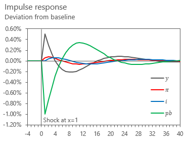
For the sake of the exercise, lets assume parameters and initial conditions for a given economy, lets name it “Country X”. Find them summarized in the table below.
To test for model stability, we check if key variables converge to their long run steady state targets, as calibrated by the model. The calibration shown above yield the following long run convergency rate for the output, inflation, policy rate and debt-to-GDP gaps:

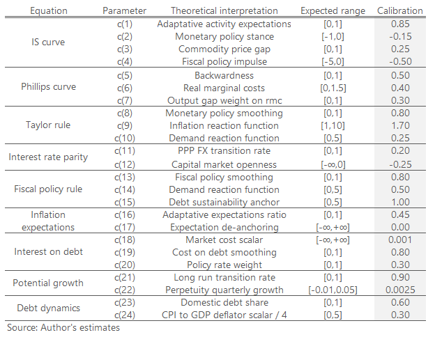
We can also check for stability and model properties by shocking our stochastic disturbances “ε(X)” and computing differences over the model benchmark. This is also known as an impulse response function. Here’s an example below using the policy rate.
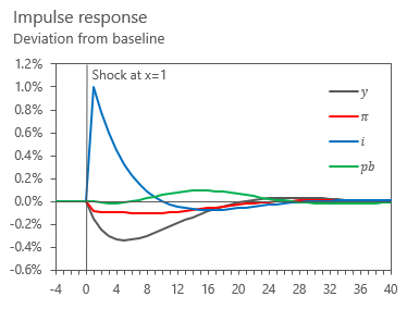
Since we’re here, lets also test the model’s response to a 1 ppt of GDP fiscal expansion shock:
A quick reversion of the output gap from positive to negative hints agents in this model to be rather Ricardian. Given that our model does not allow for spending to change potential growth in any sense, chances are that any yielding fiscal multipliers would be small, more representative of short run demand boosts, like the stylized Covid-19 pandemic relief checks, than long run public investment plans.
The model still allows for great flexilibity for fitting different economies and computing short, medium and long run responses from economic policy and more. Assuming we’re happy with the stability and economic property results of our model, we can move on to the final criteria of our calibration set and main goal of this post, which is forecasting.
Section 4: Forecasting & final thoughts
When discussing the forecasting properties of any model, it is important to contrast the different types of models available. Blanchard has a very insightful description of these in his 2017 post in the PIIE. To summarize his point, models are built to suit very specific purposes.
A model exclusively dedicated to forecasting short run inflation is very likely to exceed in accuracy models that are not specifically created for such. This would be the case of the recently developed Machine Learning tools that outperform benchmark traditional forecasting models. However, to do so, ML models often sacrifice tractability and clear storytelling capacity by relying on many nonlinear relationships and requiring gigantic datasets.
The main strength of a structural model in forecasting is its consistency. It might not be the go to tool for accuracy rankings in consensus forecast surveys, but will support a comprehensible and well-guided storytelling, precisely because it will back out all the individual transmission channels of a given forecast number. All it requires is an agreement on the equation system specification setup and the calibration assumptions, which can sometimes be fully retrieved by empirical estimates.
After testing for model stability and economic properties of an intended economy, the final test of our calibrated model is to find out if it is able to produce an output in line with consensus surveys and central bank forecasts. If your model produces a number within the interquartile range of such variables, you got yourself a perfect model to forecast and simulate with.
As it will often be the case in my future technical notes, I am leaving attached an organized spreadsheet to allow for an easy replication of all charts and results here presented. Thank you for making it this far.