Applied linear algebra in economics

VARs as toy macroeconomic models

Welcome. Today’s entry aims to explore some of the strengths of using vector autoregressive models (VAR) to simulate and forecast economies.

VAR models are useful for forecasting and scenario analysis that look overwhelmingly complicated to most due to its linear algebra presentation. So in this post I'm going to break it down into smaller and simpler steps.

To level the field about this subject, these are models that express variables that relate to each other over time as in a feedback loop. If one variable changes, a second one responds, the response of the second affects the first in a subsequent period, and so on.

To avoid excessive abstraction and motivate this topic for economists, lets give it a practical example. Think briefly about how employment, GDP and industrial production are linked together in time.

By eyeballing the chart, it is undeniable how strongly correlated these three time series are. Innovations in one are expected to lead to changes on the other two, forcing them to feed from each other. Industrial production is part of GDP and requires employment as input, on the flipside, labor demand is stronger when demand (as measured by GDP) is also strong, which pushes prices up, incentivizing an increase in supply provided by industrial production. This is the feedback loop.

We call this kind of relationship “endogenous” and the best way to represent variables endogenously is by using a vector autoregressive (VAR) model. Mathematically, a VAR(1) (1, as in one lag) model is:

Where X(t) is a (N x 1) vector of endogenous variables, A is another (N x 1) vector of intercepts, B is a (N x N) matrix of angular coefficients, X(t-1) is a (N x 1) vector of lags and V is a (N x 1) vector os shocks/innovations. If matrix algebra is not your thing, I’m breaking the matrix representation down into a system of equations below. In this example, we’re dealing with N=3.

Here, N stands for the number of endogenous variables and equations in a system that allows one lag to each variable ("x", "y" and "z"). The choice of a single lag is purely for simplication, more is certainly desirable for situations in which dynamics take longer periods to play out fully (more common cases are when one’s considering higher frequency models, such as monthly or weekly). Greek letters are parameters, these can either be calibrated to suit a given model property or estimated to fit the data.

In economics, balancing a good fit to the data without sacrificing stylized facts every economic model is expected to have is hard. This is mostly because identifying clear economic shocks is far from easy, especially when it comes to economic policy, and there’s good reason for it. This is well explained by Milton Friedman’s thermostat analogy for monetary policy. It goes somewhat as follows:

“Think about a house with a thermostat-regulated temperature. Every time the weather cools, the thermostat requires more energy to keep the house temperature stable. If the thermostat is efficient, it’d not be possible to observe a lingering correlation between the house’s inside temperature against energy consumption or outside temperature alone.

Because of lacking correlation between these time series, a naive econometrician studying the impact of energy consumption would be mistakenly led to believe that energy consumption leads to lower outside temperature, which is clearly absurd.”

Real life economists know better, and approach monetary policy in a much smarter way than the naive econometrician. If a central bank is lowering interest rates, they know its probably because it anticipates slowing activity in the near future and wants to “keep the inside temperature of the economy stable”.

Empirical estimates of VAR parameters would hardly provide an accurate understanding of such economic phenomena, even with their many different identification techniques. Thus, parameter calibration is often acceptable, and sometimes even desirable.

What I offer in this post then is a simple calibrated version of the VAR approach using three equations and one lag. I've calibrated the model in a way that it mimics the expected behaviour in interest rates (x), the output gap (y) and inflation (z). It is a toy macroeconomic model as is, but can be calibrated to suit any purpose. This is the link to the spreadsheet model. I do recommend downloading and opening it using Excel rather than Google Sheets for clearer formatting.

The black line shows simulated time series versus VAR modelled forecasts in red. These are set to mimic real life fluctuations around expected values, so that the VAR output is only accurate on average.

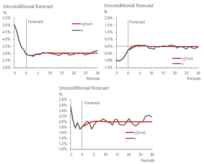
These forecasts are derived purely from the calibrated model dynamics and made up initial conditions. These can easily be changed to suit any given economy’s x, y and z variables.

VAR models are also known to allow the computation of impulse responses. These are simply differences between baseline forecasts and scenarios that impose permanent ou temporary shocks to one or more variables in the model. The spreadsheet produces the following example:

The impulse response reads as follows: a temporary 1% jump in inflation (z) forces a 0.45% jump in interest rates (x) for multiple periods, leading to a 0.3% correction in output (y) that helps inflation fall back to its unconditional average of 2%.

This is it for today’s entry. Thank you for making it this far and I hope you liked it.