


Dynamics in macroeconomics
Going beyond the limitations of comparative statics

Welcome. Today’s post is a more technical take on general understanding, teaching and modelling approaches to macroeconomics. It is about how mastering model dynamics changes the way we see the field. Let me explain why.
Motivation
At the undergraduate level, economists are taught simple linear relationships between macroeconomic variables. Put simply in an example: output is demand, more demand translates into higher employment, which leads to inflation, followed by central banks increasing policy rates, and so on.
Classic models were most often represented in those terms, and economic policy impacts approached the same way. So much so that a considerable amount of macroeconomic training is still done using two-stage diagrams and comparative statics. Recall the IS-LM-BP model:

It is certainly useful to learn the expected short run consequences of a fiscal expansion to economic activity ‘Y’ and interest rates ‘r’. Two-stage diagrams from such models cut short a good amount of abstraction in order to teach important macroeconomic concepts. A fiscal policy shock increases domestic demand, which also increases demand for imports, forcing interest rates up to support the balance of payments and stabilize dollar outflows. The near-term outcome of a tax cut or a new wave of government spending is an increase in output and interest rates, and if the exchange rate is flexible, it will appreciate a little bit too.
Simple, easy, job done. Or is it?
Well, let’s have a look at the actual linear relationship we find in the data:

Correlations are far from encouraging of the story told by the model. Years we see more government spending are actually the same years when output is lower. Smart academics will tell you that this is to be expected: the government is forward-looking and spends more when it sees the economy slowing, and it would have slowed even more if it wasn’t for that additional spending.
Whether this explanation is convincing or not, data by itself add a thick layer of complexity when taking simple comparative static results to make expectations about output. Professional economic forecasters ask themselves the following questions all the time: how much of current activity data reflects past policy decisions? Is that policy package from three years ago feeding through the economy still? To which direction? Are we beyond peak impact already? How should the combined effect of a fiscal stimulus and a monetary policy rate hike a year later look like? Was a given policy decision taken the result of an expectation to inflation that needed to be offset by that policy? If yes, what does that mean for future inflation and growth?
Questions like these are what make the applied macroeconomists’ work more challenging (and interesting). None of them can be addressed by simple intuitions coming from two-stage comparative statics. To even attempt an answer we need to move beyond and start thinking dynamically, and this is when the adults in the room start a conversation.
Dynamic models
The exercise that is about to follow is stored in this Excel spreadsheet. We start from the simplest dynamic model around, the basic three-equation closed economy New Keynesian (NK) setup:

The interesting feature of the NK framework is that it not only provides us with dynamics, but also frames how expectations about each of the variables ‘E(t)[z(t+1)]’ are formed. This way, we avoid situations like the one mentioned in the previous example, as a “what if a policy action was taken based on a different expectation?” question wouldn’t make sense because the model is supposed to describe exactly how expectations should have been formed. The model can be thought of as a way to represent how agents think about the economy at the aggregate level. Let’s solve it.
To simplify the algebra, we need to bring this to matrix notation, luckily we have touched upon this topic before (see here and here).
Next, we make use of Blanchard and Kahn’s 1980 algorithm:

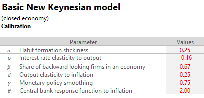
Now, we need to bring values to our parameters. This can be approached empirically, with fancy econometric estimations, or simply calibrated to hold stylized facts about the economy/country/region we’re thinking about representing here. My usual recommendation (for reasons which I’ll explain shortly) is to go with calibration and benchmark model results against consensus forecasts first, then adjust according to judgement second. This is what I got for today’s example:
We can numerically solve the model now. Following the algorithm, we can jumpstart matrices ‘K(s-1)’ and ‘M(s-1)’ using 1’s or 0’s and iterate until convergence is achieved (be mindful that bad parameter choices may not converge for reasons beyond the scope of this post).

Our model is now complete. We can study this small economy we have just created by either providing it initial conditions and studying how it develops over time or we can analyze how shocks play out. Let’s see what happens during a negative supply shock to inflation coming out from a steady state:

And what would happen if the shock came about when the economy was in the middle of a previous cycle? We can state different initial conditions and see how it would look like.
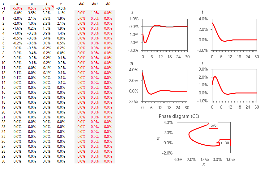
Many worthy observations can be made at this point.
Note how in the steady state initial conditions exercise the impulse of an inflationary shock is expansionary to activity at first, but contractionary for many subsequent periods later. This is a result of forward-looking agents reacting to lower ex-ante real interest rates, which requires the central bank acting sooner rather than later to support macroeconomic stabilization.
Note how in both cases the phase diagrams show a long period of adjustment between when output ‘x’ is negative, responding to central banks increasing the real interest rate ‘r’, while inflation ‘π’ is positive, only gradually normalizing from the initial supply shock.
If we were to draw a correlation from the data provided by a model that clearly specifies output to be positively correlated to inflation, we would still get a negative relationship during most of the adjustment period of a supply shock.
This is a most important fact for empirical macroeconomists. It is probably impossible to prove this model right just by observing raw correlations in the data. It should be straightforward to conclude from this that the estimates we get from purely statistical approaches understate the impact output has to inflation, and lead to faulty conclusions such as “The Phillips Curve may be broken for good”.
One last worthy note to point is how well-identified initial conditions matter for results to hold. Given that the economy is not being evaluated at its steady state in the second exercise, we see a much bigger jump to inflation (to 3.5%, from 0.5%) than in the steady state exercise (to 1.2%, from 0%), because of how well the model captures how much lower inflation in ‘t=-1’ should have been given that output was 5% below trend then. The mere rebound in activity was enough to propel inflation by an additional 2.3ppts (3.5% - 1.2%), so properly accounting for initial conditions matter just as much as shock identifications. This is a nuance comparative statics exercises wouldn’t allow us to see.
And that’s all coming from a fairly simple three-equation framework. In the spreadsheet I am also providing an extended six-equation model that covers active near-term fiscal policy, foreign sector and global interest rate shocks. It should help users figure out how to extend the model from here.
That’s it for today’s post. My main message was to show how comparative statics and simple partial derivative intuitions aren’t as useful as people seem to think when navigating real-life macro questions. Future outcomes depend on context and shock identification just as much also. Two of the many other reasons why we need to think dynamically, not statically.
This is it for today’s entry. Thank you for making it this far.