
The case for renting
An algebraic take on whether to rent or buy a home

Welcome. Today’s post is about a practical question that most households face at least once: are we better off living on a rented home, or should we look to lock a mortgage and buy our first property to move in as quickly as we can?
I know how exhausted this question has been over the years, but what I promise here is something slightly deeper than just a conclusion. This is the best way to frame this question logically I could come up with so far. This post will be rather technical, but I hope to convey a lot of complex information into a small set of equations.
Before we begin, it is important to note that a home is ultimately a durable good. As such, it should be viewed as something that households consume, not necessarily invest in, so comparing which decision results in making the most amount of money is not completely fair here. People take satisfaction in owning a property, with all the benefits and liberties that come from it. As far as this is concerned, I don’t personally believe there is an objective price for the “happiness” of consuming something.
Economists, however, are known for measuring “happiness” as opportunity costs of people’s decisions. This post is about that. If you are already set on owning a home, the goal is to inform you how much future wealth you would give up to do so. Think of it as a value for how “happy” your decision makes you feel.
This exercise is detailed in the attached spreadsheet. So without any further ado…
The assumptions
Let’s state some basic assumptions to set the stage. The story goes as follows:
One agent with enough savings for a down payment on a mortgage is considering if he(she) should…
Buy a house, replacing rent costs for a mortgage; or
Keep living on a rent and invest all savings on a market portfolio instead.
We want to know how much wealth is accumulated by the end of the N months of a mortgage in each scenario, and then compare.
By appropriately defining the problem we can find how to assemble the moving parts of each decision.
The home buyer’s wealth
The home buyer’s wealth at period ‘N’ is driven by the following equation:

Where ‘w(h)’ is the home owner’s wealth, ‘p(h)(b)’ is the house price at purchase, 'g(hp)’ is the expected growth rate on the house price over time, ‘t(p)’ is the property tax rate (diluted across the mortgage repayment period), ‘d(h)’ is the linear depreciation rate of that home, ‘m’ is the monthly payment on the mortgage (which is a function of the price of the house, the down payment ‘d’ as share of that house price and the interest rate on the mortgage ‘i(m)’), lastly, ‘π’ is the consumer price inflation rate.
To simplify this problem considerably, we can abstract inflation away by denoting all our parameters as values adjusted for consumer price inflation (so all rates are above that of inflation and all values constant monetary units at the time of purchase of the home). Our final equation for the expected wealth of a home buyer is:

This equation can be described as follows: the wealth of the home buyer in the future will depend positively on how much the house price grows, negatively on how much it will cost to maintain it due to taxes and depreciation and also negatively on how much he will pay for the loan to acquire it.
We need to break the mortgage down a little further, so allow me to explain how mortgages work algebraically as well. If you want to simply trust me, feel free to skip the interlude below.
Interlude 1 - Debt, interest rates & amortizations.
A mortgage is a simple debt that yields compounded interest rates and work on constant amortization schedules. If we know the size of the debt, how much interest it yields and for how long we are going to pay it for, we can calculate the size of the periodic amortizations. It goes like this.
Suppose debt ‘D’ is taken at time ‘t’, at a ‘i(m)’ interest rate, negotiated to be amortized by the amount ‘m’ paid over ‘N’ periods. This debt will evolve as follows:

At rearranging terms at time ‘t+3’ to back out values as function of the initial debt stock, we can notice a pattern that can be generalized to:

Where the second term in the right hand side of the equation is a finite sum of a geometric series. Which boils down to:

Since we know that this debt has to be paid in full by the ‘Nth’ period, we can make so that ‘D(t+N)=0’ and solve for ‘m’.

This is the general formula to determine the monthly payment of a debt. If we plug in the debt stock as the price of the house minus the down payment for the mortgage, we end up with
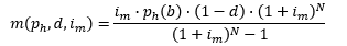
Which is exactly our mortgage payment for the home buyer’s wealth.
We can now move on to the other side of our rent(buy) problem, the renter+investor.
The renter+investor’s wealth
By choosing not to borrow money to acquire a property, the renter+investor’s wealth ‘N’ periods from his decision day should be driven by the following equation:

Where ‘w(r)’ is the renter+investor’s ending wealth, ‘i(inv)’ is his net of fees & taxes average investment returns and ‘b’ is the rent he would pay on a comparable home. We can further simplify this equation by substituting the second term on the right hand side of the equation for the solution of the sum of the terms in a finite geometric series.

Explaining this equation in plain English, it states that the wealth of the renter+investor will depend on the initial investment, that is, the down payment he(she) would have saved, plus the periodic contributions he(she) would add to his(her) portfolio for opting to pay for a rent instead of a mortgage, both accrued over the counterfactual loan period by an average market investment return.
It is also important to note at this point that home prices and comparable rents are not independent from each other. In fact, rents are a key component for determining the price of a property. This warrants a second (and last) interlude.
Interlude 2 - Home prices & rents
Home prices can be valued in a few different ways. The one we’re going to use is the intrinsic valuation method. A house price is defined by the present value of an infinite stream of future cashflows associated to the land and its facilities.
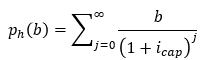
Here, house price ‘p(h)(b)’ depends on an infinite sum of periodic rent value ‘b’ discounted by a capitalization rate ‘i(cap)’. This capitalization rate is a required rate of return by the real estate market to invest in a given property.
The right hand side of our equation is the classic infinite sum of a geometric series of ratio ‘(1/(1+i(cap))’, which can be solved analytically to become:

Which is topped up by the property tax, paid once during the home acquisition. This is the final formula that links home prices to rents.
We are done describing the renter+investor’s wealth. Next, we piece everything together.
The opportunity cost of buying a home
It is time to bring our algebra into feasible numbers. To compare the accumulated wealth in each scenario, we make use of a simple formula:
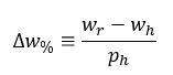
Which will state the difference in accumulated wealth as a share of the house price acquired 20-years prior.
Next, we calibrate each parameter with reasonable numbers. Here, I am aiming to describe the London real estate market.

Our parameters translate into a £499,220 (£874,004 - £374,784, or 54% of the initial house price) in additional wealth accumulation over 20 years. A material amount. This value, however, can be significantly different if we move some assumptions around.
What if one is a terrible investor or has an excellent eye for good property/land value? We can see what happens if we assume different investment returns or price growth rates.

There seems to be a scenario where the home owner would actually make more money than the renter+investor. Especially if the investor isn’t diligent with his(her) savings or invests it poorly, making near-zero returns over his wealth accumulation period.
Let’s run a second sensitivity analysis. What if one has access to cheap financing or chooses a region with vastly different depreciation rates? We can see what happens if we consider more/less attractive interest rates on a mortgage or slower/faster depreciation rates on the land acquired.
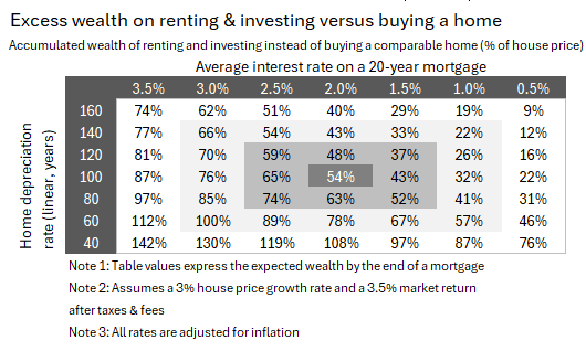
Higher depreciation rates can translate into a rent/buy wealth wedge just as material as making great investment returns. Home buyers should be aware of risks associated to what a bigger exposure to natural disasters, poor public service and related matters do to their land value.
Concluding thoughts
I hope the reader is convinced that this was no ordinary rent/buy take. The spreadsheet should allow readers to adapt parameters to their personal circumstances and reach their own conclusions.
This is it for today’s post. Thank you for making it this far.