The mathematics of retirement planning

Simple algebra from financial mathematics

This entry comprises a good amount of algebra, where I explore known financial mathematics derivations to explain how retirement plans (401(k)’s and such) work. This post assumes all financial operations to be made under compounded interest rules, as it is common practice for long-term borrowing/lending (still, it should be easy enough to adapt this framework to simple interest whenever applicable). Moreover, all monetary flows in this exercise are considered to be ​​adjusted for inflation and net of any costs and taxes, therefore returns are also expressed in post-tax real terms accordingly. This simplifies the algebraic representation of our cashflows.

To make things easier, we should split our retirement plan into two fundamental stages: the first stage comprises the capital accumulation phase whilst the second comprises the retirement phase when a given worker forfeits his income from labor and can only consume the wealth accumulated during the first phase.

Step 1: Capital accumulation

In the capital accumulation stage, the saving worker decides on a fixed amount of constant $ to be saved in each period (the fixed amount is also convenient for simplicity, but you could assume it as a period average too). During retirement, accumulated wealth will be our saver’s only source of funding for consumption after retirement. Let us then state some of our assumptions:

1. Our representative worker lives with an average real income ‘Y’ until retirement after ‘t1’ periods (let’s talk months from now on);

2. During the capital accumulation period the worker saves a constant $ amount defined as ‘s’ every month;

3. Savings are immediately fully invested in an asset/portfolio yielding real average monthly returns ‘r’.

If we define ‘S’ as the future value of our invested capital, we know that:

Here, we sort the contributions in chronological order. The first contribution will earn interest for a longer horizon, which then means it will have more weight on final accumulated wealth.

‘S’ is also known as the sum of the terms of a finite geometric progression (therefore a geometric series, GS), a sequence of numbers whose elements are multiplied by a common ratio ‘q’. There is a very elegant way to represent the sum of all the finite terms in such a series:

Where ‘a1’ is the first term of the GS, ‘q’ is its ratio and ’n’ is the qty of terms

This formula greatly facilitates the work of calculating the accumulated future capital, as we can do so simply by substituting our known elements. ’n’ equals ‘t1’, ‘q’ can be represented as ‘(1+r)’ and ‘a1’ should then be ‘s(1+r)’ by consistency. We then have:

We can finally simplify the equation as follows:

Thus, we arrive at our final equation for the accumulated equity as a function of the amount saved ‘s’ yielding a given expected real rate of return ‘r’ for ‘t1’ months.

However, one question comes to mind. What is the ideal size of equity to accumulate? What if we accumulate too much, sacrificing more consumption than we would like for savings we don’t need, or too little, sacrificing more consumption at old age instead or worse, not being able to afford fundamental care?

The retirement step of our retirement planning will help us figure this out.

Step 2: Retirement

The retirement stage begins in the month following the representative saver’s last working day. Let us then state a new set of assumptions:

1. The worker will monthly redeem a real fixed amount ‘A’ from its savings for ‘t2’ months, based on his post-retirement life expectancy;

2. The remaining unredeemed capital continues to yield the same real expected return from our previous capital accumulation step, ‘r’;

3. Savings are to be fully consumed in monthly installments (therefore allowing us to define how much accumulated capital is required).

To facilitate the interpretation of our exercise in this step, we can think as if we were the saver’s counterparty, most often a bank or other kind of financial institution (pension/hedge fund) that borrowed our saver’s money in exchange for a future expected return ‘r’. This counterparty’s debt, defined as ‘P’, then yields the following present value:

As in the previous step, we have another case of geometric series. This one has a ratio ‘q’ equal to ‘1/(1+r)’ and ‘a1’ equal to ‘A/(1+r)’. We then apply the finite sum of a geometric series formula again:

Once again, we can simplify our equation as follows:

If we want to find out the value of the amortization installments of this debt, we can solve for A:

Debt amortization equation. Alternatively, we can think of ‘A’ as the value of a monthly pension benefit to be consumed from the accumulated savings ‘P’

This last equation is a well-known mathematical formula result, useful for calculating debt repayments under constant amortization schedules and widely applied by banks to analyze a borrower’s repayment capacity after income checks. Here, however, we will give it a different interpretation: it is set to become our saver’s monthly average income after retirement. This should be made clearer in our next (and final) step.

Step 3: Piecing 1 & 2 together

Now, we are going to join steps 1 & 2 by equating ‘S = P’. Note that in our previous steps we were careful enough to represent ‘S’ & ‘P’ as $ amounts of the same period, which is the month when the retirement period begins.

Let us simplify this algebra:

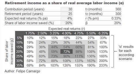
With this, we find ‘A’, a fixed constant $ amount of monthly debt repayments which amortizes an accumulated debt of the counterparty that must be paid to the saver in ‘t2’ months. ‘A’ is exactly a social security benefit that our retiree will redeem periodically for the planned period of ‘t2’. ‘t2’ is most often defined as the additional number of months an individual expects to live after his retirement. As an illustrating example, we can also choose to express ‘t2’ in years, assuming that our saver retires at 65 years of age and assumes to make until 90 years old, ‘t2’ = 90–65 = 25 years (or simply, 300 months).

In a final step, we can make some useful definitions using ‘A’ and ‘s’ as shares of our saver’s real average income:

So that ‘α’ is the retiree’s income as a share of their average real income (also known as retirement replacement ratio) and ‘β’ is the share of the real average income saved during the period of capital accumulation (his savings rate).

With this final equation, we arrive at our intended result. We can simulate infinite scenarios for the retirement replacement ratio ‘α’ as a function of the share of income that our agent saved on average ‘β’ over ‘t1’ months, which he should receive for ‘t2’ months after he decides to retire, which also depends on the actual average rate of real returns ‘r’ of his investments. Using this formula, I’ve simulated a couple of potential outcomes in the matrix below.

Final thoughts

It is amazing what can be done with simple algebra borrowed from known derivations of financial mathematics. As a previous pension fund investment analyst, I can attest that these steps summarize the bulk of the financial planning involved when it comes to calculating the average saver’s pension benefits. From now on, you can do it yourself.

I am leaving the reader with a public spreadsheet with all the algebraic steps and the simulations here presented for those who might be interested or may want to redo the exercise based on their own parameters. Find it attached in this Google Drive link.

That would be all for today’s entry. Thank you for making it this far.