


Applied linear algebra in economics - part 2
An empirical application of VARs to uncover latent variables

Welcome again. In the first post on this topic we explored vector autorregressions (VARs) as means to simulate and forecast economies. Today, I am going to use them again in an empirical application: the estimation of what economists call the neutral interest rate.
Neutral rates
To start simple, lets briefly explain what the neutral interest rate is.
As keepers of inflation, central banks aim to gauge the economy’s liquidity (amount of money in circulation) and domestic demand (GDP growth) at a level consistent to an inflation target provided to them. In the case of the United States, the Federal Reserve is instructed to target a 2% average inflation rate while keeping the economy running at a balanced growth pace (also known as full employment). It does so mainly by calibrating a basic interest rate that feeds through the rest of the economy, the Fed funds rate.

But how can the Fed know how far it can push the Fed funds rate to achieve that 2% average inflation target without hurting or overstimulating the economy? It has to start from a baseline, a reference point. One way of gauging that reference point is to find what would be the apropriate basic interest rate if the economy was already at full employment with a 2% inflation rate. This is what economist’s mean when they talk about the neutral interest rate.
In short, the neutral rate is this balanced, yet unobservable, policy rate that keeps the economy in “a steady state”, stable around the central bank’s objective. And knowing this neutral rate helps to guide central banks fine-tune its policy stance. If the economy is running a little hotter/colder than usual and inflation is above/below the target, they move the basic rate above/below that neutral rate. This way, they steer the economy back to where it is supposed to be.
We now know that the neutral rate is sort of a baseline for the policymaker. But finding that baseline is tricky though, as any economy is comprised of multiple moving parts that feed from each other as in a big feedback loop.
If you recall the previous post, this should ring a bell. VARs are suited to model exactly that. In this post, I am going to provide a barebones estimate of the US neutral interest rate from this method. The exercise was entirely done in Excel using FRED data, and the spreadsheet link can be found here.
Empirical strategy
The model used is a simple VAR(1), same as the one used in our previous post.
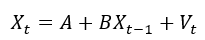
Where X stands for a vector of seven endogenous variables, comprised of the Fed fund effective rate, bond yields across four different tenors, PCE inflation and industrial production as a proxy for economic growth. A is a vector of intercepts, one for each endogenous variable. B is a 7x7 matrix of angular coefficients. X(t-1) is the same as X, only lagged one period. Finally, V is a vector of shocks, assumed to be white noise.
The use of bond yields in the context of this exercise is because the bond market carries an important component of forward looking expectations to it, an important ingredient to offset the fact that much of our data could be a fairly weak signal of the future.

Markets trade in yields what they think will happen to the Fed funds rate based on how they see future economic growth and inflation. Its not a perfect proxy for expectations of interest rates for reasons too complex to discuss in this post, but useful nonetheless.
The idea here is to estimate a rolling sample VAR across 1985 to 2024, using monthly frequency data. The coefficients of these estimates can then be used to compute a long run expectation for each endogenous variable, like so:

If the long run expectation of each of the variables are consistent with an inflation rate close to 2% on average. If it isn’t, then we can simply recalibrate all long run coefficients to lock for what would be consistent to a 2% long run inflation expectation with a scalar multiplication. Then, we are safe to conclude that the yielding long run expectation of the Fed fund rate is a good approximation of the neutral rate. Let’s exemplify below.
Results
Lets use a full data example. Regressing all data from 1985 to Jan/2024, we yield the following:
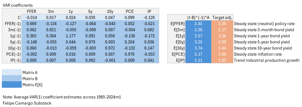
Doing the matrix operations shown above and then adjusting the (I-B)^(-1)*A vector to back out a consistent 2% long run inflation expectation multiplying the yielding long run coefficients by a scalar 2/2.17, we find that 2.26% would be a reasonable approximation of the neutral interest rate from our full sample.
However, we should not stop there. From eyeballing the chart, we know interest rates have trended down over time, maybe we can capture regime changes in the neutral rate over time using a rolling sample. By repeating this exercise using rolling 180 months (15 years) of data, we come across the following chart.

We should find that although the average of this moving neutral rate isn’t that far off from the full data sample estimate (about 2.7%), data at the margin is considerably different. The neutral rate has trended down until the pandemic crisis, shifting into an upward trend from 2021 up the last data point, to 1.4%.
How to improve from here
How plausible are these results? Its important to note that this was all built on a single weekend in one Excel tab. There’s certainly room to make this much better. Lets number a few ways in which we could improve further from here.
VARs are often overparameterized, meaning that they require an excruciating amount of data to yield stable/reliable results. The reason why I chose industrial production, rather than employment, retail sales or the unemployment rate as a proxy for economic growth is because it was the only of these that provided sensible results without big structural breaks during the Global Financial Crisis (GFC) or the Pandemic Crisis (PC). This leads into two problems which I think pushes a downward bias in our neutral rate estimate.
One is the need to average rolling estimates across a much bigger (fifteen years is too much!) horizon. For most of the last fifteen years period inflation was below target and the Fed practiced Quantitative Easing (QE), having only recently moved into a tightening instead. We are potentially not capturing this regime shift as well as we could, although bond yields could be controlling for some of this.
The need for more data limits us to bring this exercise into quarterly frequency, where we could have relied on crude GDP numbers which are probably the most relevant metric for economic activity available. It is important to note that the US is a much more services-oriented economy now, and having lower industrial production growth rates is just a part of that.
To fix for this problem, we would probably benefit from Bayesian statistical techniques that allow us to shorten the need for data in our estimates. This is better addressed in Appendix B here.
We are not appreciating any economic theory here. Our exercise was nearly purely empirical and fails to account for stylized facts of a given economy. Methods that successfully marry theory to data such as the one provided by the NY Fed tend to be the most informative, as they are structured in a way that is consistent with a lot of other factors just as important, such as productivity, consumer preferences, demand and supply for investable assets, and so on.
Final thoughts
The goal of today’s post was to share further practical knowledge on VAR models with an application. I find these to be missing from most econometrics classes I know, especially in accessible languages such as Excel.
Important note: This post was updated with a second version which includes the scalar adjustment to lock long run inflation expectations at the 2% inflation target. The spreadsheet was also changed, you can redownload the newer version from the previous link.
This is it for today’s entry. Thank you for making it this far and see you in the next one.