


Fiscal policy analysis - a macroeconomist's guide. Part 1 of 2
Algebraic tricks for the everyday fiscal policy analyst

In this entry, I explore simple yet effective methods for analysing fiscal policy. These apply for both cross-country and time series assessments, and I think should be in every fiscal policy enthusiast’s toolkit.
What comprises “fiscal policy analysis”? Everything that relates to fiscal budgets, government balances and public debt. Fiscal policy is one way governments intervene in the economy, and is the unavoidable part of every public sector’s existence.
Fiscal policy collects taxes and issues debt to spend it back in the economy in many different ways. Public spending examples range from state owned enterprises (SOEs), Public-Private Partnerships (PPPs), public infrastructure projects, transfers and, naturally, its own body of employees.
Fiscal policies have multiple objectives, but most often they aim to stabilise economic cycles, support long run growth, reduce poverty and inequality, basically tackling distortions created by market failures the best way it possibly can.
Though whatever the objective, all sovereigns face budget constraints. Though it may not be as rigid as a household constraint, as governments often have sovereignty over its own currency, which allows them to issue their own debt and control the rate of inflation under which previously issued debt is subject to. There are many examples of the use of inflation to avoid local currency defaults, but thats certainly more of an exception. Most governments pay their debts while keeping inflation under control, and this will be an important assumption through today’s analyses here.
But enough of Google search talk about it. This post aims to show a couple of useful algebraic takes to either better understand fiscal policy and/or analyse it with some deeper insight.
Take 1: The fiscal spending multiplier
The fiscal spending multiplier is an useful concept for macroeconomists, it states how much we should expect an economy (Y) to grow after a change in government spending (G). There are multiple formulations for this, but here I’ve decided to stick with a more classical version with my own adaptation.
Starting from the fundamental expenditure-side GDP identity:
From here, we can reestate all level variables as percentage point contributions to the GDP growth rate, like so:
Where ΔY(t)/Y(t-1) is the GDP growth rate, while ΔZ(t)/ΔY(t-1) stands for the “Z” expediture-side component contribution to GDP growth. To make things easy, we can simplify component contribution notations further by defining ΔZ(t)/ΔY(t-1)=z(c).
From this point, we can assume behavioural equations for the right hand side variables of our GDP growth identity. I’ll state them all at once and then explain each.
Our behavioural equations state the following:
Household consumption contributions “c” depend on the autonomous consumption rate of change “α0”, a marginal propensity to consume “α1” over past change in disposable income “(1-Δτ)y(t-1)”, also being negativelly affected by an elasticity “α2” to the real interest rate “r”.
Government consumption is exogenous, assumed to be dictated by the government.
Investment depends on autonomous investment “β0” but is also negativelly affected by a “β1” magnitude by the real interest rate “r”.
Exports are also assumed exogenous, being a function of external demand which is not controlled by any domestic agent.
Imports follow a similar behaviour as household consumption, except it depends on disposable income adjusted by changes to the real exchange rate “q”.
To account for a “crowding out” effect, we should also assume that increased spending increases the interest rate and affects the real exchange rate.
Since both “g” and “r” affects the real exchange rate at the same time in opposite directions, we should back out the net effect of "g” into “q”. Substituting the “r” equation in the right hand side of “q”, we get:
Now, we can finally substitute all behavioural equations into our GDP growth formula:
Where “ψ0” simplifies:
We can then solve for “y” as a function of “g”.
And in a last step we can finally back out our multiplier by taking the partial derivative of “y” with respect to “g(bar)”.
Despite all the work, this formulation of the fiscal multiplier is advantagenous for a number of reasons.
The first one is that it forces the analyst to account for most of the ingredients behind the impact of an increase in public spending to GDP.
Lets start from the numerator. The “δ2(λ1-λ2γ1)” term expresses the exchange rate impact to the fiscal multiplier, if government spending depreciates de exchange rate, then it is expected the multiplier to be higher, as this will reduce a negative spill over effect driving domestic demand to foreign goods. Meanwhile, the “γ1(α2+β1)” term represents a “crowding out” effect of public spending. By increasing spending, agents can foresee an increased need in increasing the supply sovereign debt, which will therefore affect the interest rate positively, making the expected credit for household consumption and investment more expensive.
Now, the denominator. “α1-δ1” represents the net marginal propensity to consume domestically, that is how much will households consume in an aggregate for an additional unit of income from a government transfer. Meanwhile, “1-Δτ” gauges the impact on increased spending on income taxes, how much they are expected to increase in order to fund further spending.
The second advantage is that this can be easily calibrated to fit any economy. Lets consider the following numbers:
𝛼1 = 0.50, 𝛼2 = 0.10
𝛽1 = 0.15
𝛿1 = 0.30, 𝛿2 = 0.75
𝛾1 =0.20
𝜆1 = 5%, 𝜆2 = 3.5%
∆𝜏 = 1%
This would yield a fiscal multiplier of 1.22, which means that every unit of additional government spending is expected to return 0.22 over the amount spent in additional GDP. Quite amazing, right? But this is only because the economy is fairly closed off to imports and the marginal propensity to consume domestically is high. If we change this assumption gradually holding everything else constant, we get the following chart.
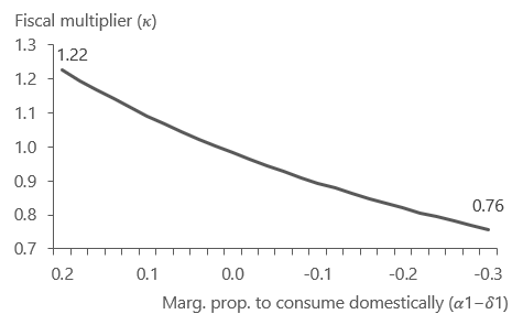
An increasing amount of imports an economy incurs over domestic consumption reduces the fiscal policy’s ability to stimulate the economy.
Lets now consider the crowding out factor. Recall briefly that this is the positive effect that spending has over interest rates, which affects household consumption and investment negatively. Risks associated with how high the debt burden of the sovereign is will affect this variable. Once again holding all else equal we get the below.

Either a higher sensitivity of the interest rate to increased public spending or an increased sensitivity of the domestic economy to interest rates will also reduce the ability of the sovereign to steer the economy with additional spending.
Hence we have deduced a useful way of thinking about spending multipliers. This can then be used to inform expectations on GDP growth and further analyses regarding fiscal accounts. The spending multiplier will be a key ingredient for our next fiscal take.
Take 2: The primary balance elasticity to spending
Most analysts tend to look at fiscal balances as accounting exercises, in this take I’ll show how this is not entirely accurate. From the previous exercise we know that public spending has an impact to activity via the fiscal multiplier. The latter should in turn affect government by boosting tax revenus, hence assuming that the impact of changes to spending “G” to the primary fiscal balance “PB” being a 1-to-1 relationship is rather a stretch.
To back out the expected impact of spending to the primary balance taking into account the revenue transmission channel, we can start from an accounting identity:
Where “T” stands for government revenues. Since we know that revenues are a function of economic activity “T(Y)” (where “Y” is the nominal GDP) and activity is a function of government spending, we can safely assume that T is a function of G, “T(G)”.
From this starting point, we’re looking into bringing the exact effect spending has on public revenues formally. We can start by diving both sides of the equation by “ΔG”.
Next, we divide and multiply the fraction on the right hand side of the equation by “ΔY” and rearrange, like so:
We know “ΔY/ΔG” from somewhere, don’t we? But lets not stop here. Again for the algebraic trick, we’re going to divide and multiply that same fraction by “T” and “Y” and then rearrage one more time.
Here, we can introduce a new fiscal accounts concept, the “fiscal revenue elasticity to GDP”. The concept holds that there’s a clear relationship between how much the economy produces and how much the government is able to collect, be it taxes, contributions or charging for SOE services. The revenue elasticity to GDP is defined as:
Which is already apparent in our previous equation. We can also recall the other well known identities in our right hand side term: “T/Y” is an economy’s tax burden, while “ΔY/ΔG” is the spending multiplier. We can define “T/Y=τ” and “ΔY/ΔG=κ” and substitute in the second to last equation to get:
Which therefore defines exactly the interaction between changes in spending “ΔG” and to the primary balance “ΔPB”. The spending impact on the primary balance depends on (1) how much the government costs to the economy “τ”, (2) how much it impacts the economy when giving back in spending “κ” and (3) how much it collects back when the economy grows “ϵ”.
Since tax burdens “T/Y” are often stationary within a given mean across time in most economies, we can hold it fixed at a country’s given historical mean and analyse how different calibrations of “κ” and “ϵ” affect the impact of spending on the primary balance. Assuming a tax burden of 40% of GDP, we can draft the following table:

With this, we show that an economy with a high 1.2 fiscal multiplier that also charges 40% of its domestic product in taxes is able to reduce its primary balance by about half of its increase in spending. Analysing the table horizontally we can gauge the impact of the spending multiplier, while vertically the impact of the GDP elasticity to public revenues. The higher they are, the lower the negative impact spending has on the fiscal balance.
If you are looking to forecast fiscal accounts based on government spending package announcements, you can look for IMF, OECD, World Bank and central bank estimates for both the spending multiplier and the revenue elasticity to GDP on recently published papers all around (see here and here).
Concluding thoughts
In this post, we’ve discussed two useful algebraic tricks to better understand some macroeconomic relationships between growth, public spending and the fiscal balance. In the first take, I’ve shown an intuitive way to think about the spending multiplier, while in the second the impact of said multiplier has on the fiscal balance, tax burdens and fiscal revenue elasticities to GDP considered.
This is the first of a two part post I’m planning for this blog. Find the second part in this link. Thank you for making it this far.
Você usou DeltaX(t) para denotar a variação das "exportações" e as variações de todas as variáveis do lado da despesa. Fica confuso para os leigos.