Fiscal policy analysis - a macroeconomist's guide. Part 2 of 2

Algebraic tricks for the everyday fiscal policy analyst

Hello again, this post is the second and final of a two-part entry I started last week. Make sure to check the previous one for context. The idea of this series is to share some useful fiscal policy insights using simple algebra.

I’ve left this second part to briefly discuss algebraic decomposition ideas for both the fiscal balance and public debt. Decompositions are useful ways of breaking down the drivers of a given identity-based number each year, allowing for a more nuanced narrative across time.

Given how big fiscal numbers are, it is good practice to either normalise them by inflation (therefore comparing them as constant monetary units of a given year) or by GDP, with the former being more common than the latter.

Lets get to it then.

Take 3: Decomposing fiscal balance movements

\(\Delta fb_t = \Delta t_t - \Delta g_t - \Delta int_t - \pi_t^{effect}-\delta_t^{effect}\)

The sole motivation of this take is to deal with the fact that fiscal balances as shares of GDP are quite boring. Boring in the sense that revenues, primary spending and interest payments are often stationary (mean reverting) with not enough volatility over time. Here’s a chart for “country X”:

Just by looking at the chart itself, it isn’t easy to tell what is exactly changing each year by eyeballing bar sizes in revenues and expenditures and back how public balances moved as they did. In order to find that out, we can take the first difference of the fiscal balance and decompose its movements, like so:

The second chart shows the decomposed fiscal balance movements from the same country shown in the first chart. This to me is a clearer representation of what components of the fiscal balance are driving balance changes within each year.

To build such a chart, we need to work the fiscal balance as below. Starting from the fiscal balance identity:

\(FB_t \equiv T_t - G_t - {INT}_t\)

To follow the usual standards for fiscal balance analysis, lets divide both sides by the nominal GDP (price level times real GDP “PY”) and define the absolute change to fiscal balance as a share of GDP.

\(\frac {FB_t} {P_t Y_t} - \frac {FB_{t-1}} {P_{t-1} Y_{t-1}} \equiv \frac {T_t - G_t - {INT}_t} {P_t Y_t} - \frac {T_{t-1} - G_{t-1} - {INT}_{t-1}} {P_{t-1} Y_{t-1}}\)

Next, we should define that the price level grows at the inflation rate “π” and the real economy grows at the growth rate “δ”. By assuming this we can now rewrite the right hand side of our equation as:

\(\Delta \frac {FB_t} {P_t Y_t} = \frac {T_t - G_t - {INT}_t - (T_{t-1} - G_{t-1} - {INT}_{t-1})(1+\delta)(1+\pi)} {P_t Y_t}\)

We can distribute the products in “(1+δ)(1+π)” to get “(1+δ+π+δπ)” and then take “(T-G-INT)” out of the factoring to obtain changes in the fiscal account components, like so:

\(\Delta \frac {FB_t} {P_t Y_t} = \frac {\Delta T_t - \Delta G_t - \Delta {INT}_t - (T_{t-1} - G_{t-1} - {INT}_{t-1})(\delta +\pi + \delta\pi)} {P_t Y_t}\)

At this point, we can split fractions once again and define “Z/PY=z” to save some notation.

\(\Delta fb_t = \Delta t_t - \Delta g_t - \Delta {int}_t - \frac {(T_{t-1} - G_{t-1} - {INT}_{t-1})(\delta +\pi + \delta\pi)} {P_t Y_t}\)

We can also rewrite the denominator back to (t-1) again using growth rates to get “fb(t-1)”:

\(\Delta fb_t = \Delta t_t - \Delta g_t - \Delta {int}_t - (\frac {\delta +\pi + \delta\pi} {1+\delta +\pi + \delta\pi}) fb_{t-1}\)

Finally, we can split the numerator to get the inflation “(π+δπ)” and growth “δ” effects from our decomposition.

\(\Delta fb_t = \Delta t_t - \Delta g_t - \Delta {int}_t - ([\frac {\pi + \delta\pi} {1+\delta +\pi + \delta\pi}]+ [\frac {\delta} {1+\delta +\pi + \delta\pi}]) fb_{t-1}\)

And finally we can just rebrand the odd fractions to obtain our final equation:

\(\Delta fb_t = \Delta t_t - \Delta g_t - \Delta int_t - \pi_t^{effect}-\delta_t^{effect}\)

Hence, we obtain decomposed movements of the fiscal accounts, which allows us to more easily identify drivers for changes to the nominal balance within periods. These changes hold at an identity, and periods can be measured in all possible frequencies allowed by data availability.

Take 4: Decomposing debt creating flows

\(\Delta d_t = (\frac {r_t^w} {1+\delta_t})d_{t-1}+(\frac { \alpha_{t-1} [1+r_t^w]\epsilon_t} {1+\delta_t})d_{t-1}-(\frac {\delta_t} {1+\delta_t})d_{t-1} - pb_t + \varepsilon_t\)

In this fourth and final take, I should dive deeper into debt sustainability analysis algebra. This take will account for most of the required steps for one to assess gross public debt at its most general case, as this will be required for decomposing the different possible sources of debt creating flows.

As usual, we start simple by stating identities. Public debt is the sum of domestic and dollar denominated debt.

\(D_t \equiv D_t^d + s_tD_t^f\)

Where “s” stands for the nominal exchange rate over the US dollar (LCU/USD).

Next, we need to state the law of movement for each kind of debt. That’s when interest rates and the primary balance come into play.

\(D_t \equiv D_{t-1}^d+i_t^dD_{t-1}^d + s_tD_{t-1}^f+i_t^fs_{t-1}D_{t-1}^f+G_t-T_t\)

Definiting “ϵ” as the depreciation of the exchange rate, we can rewrite the previous equation as follows.

\(D_t = (1+i_t^d)D_{t-1}^d + (1+\epsilon_t )(1+i_t^f)s_{t-1}D_{t-1}^f+G_t-T_t\)

We can now divide both sides by the nominal GDP, again states as “P” times “Y” for the price level and the real output.

\(\frac {D_t} {Y_t P_t} = \frac {(1+i_t^d)D_{t-1}^d +(1+\epsilon)(1+i_t^f)s_{t-1}D_{t-1}^f} {Y_t P_t}+\frac {G_t-T_t} {Y_t P_t}\)

At this point, we can rewrite local currency and dollar denominated as simple shares of total debt using the letter “α” to represent the share of dollar debt, like so:

\(\frac {D_t} {Y_t P_t} = \frac {([1+i_t^d][1-\alpha_{t-1}] +[1+\epsilon_t][1+i_t^f]\alpha_{t-1})D_{t-1}} {Y_t P_t}+\frac {G_t-T_t} {Y_t P_t}\)

As we have done multiple times in previous takes, lets define real GDP growth and inflation as “δ” and “π”, respectively, and define variables as percentage points of GDP in lower case letters “Z/YP=z”. Recall also that “T-G=PB”. We yield:

\(d_t = (\frac {[1+i_t^d][1-\alpha_{t-1}] +[1+\epsilon_t][1+i_t^f]\alpha_{t-1}} {(1+\delta_t)(1+\pi_t)}) d_{t-1} - pb_t\)

We’re getting there, only a couple of fixes left. Since we often can’t observe how much of interest was paid on each kind of debt, lets simplify interest on debt further by stating that total interest payments are, by approximation, a share of previously issued debt. Hence we can state a weighted average interest rate on debt for both local currency and dollar denominated debt stocks, as follows:

\(d_t = (\frac {[1+i_t^w][1-\alpha_{t-1}] +[1+\epsilon_t][1+i_t^w]\alpha_{t-1}} {(1+\delta_t)(1+\pi_t)}) d_{t-1} - pb_t\)

\(d_t = (\frac {([1-\alpha_{t-1}] +[1+\epsilon_t]\alpha_{t-1})[1+i_t^w]} {(1+\delta_t)(1+\pi_t)}) d_{t-1} - pb_t\)

And now we can use the Fisher equation to abstract inflation rates away and get the weighted real interest rate on debt “r(w)”.

\(d_t = (\frac {([1-\alpha_{t-1}] +[1+\epsilon_t]\alpha_{t-1})[1+r_t^w]} {1+\delta_t}) d_{t-1} - pb_t\)

The above equation is an interesting starting point to create debt forecasts and assess sustainability under certain scenarios for “r(w)”, “ϵ”, “α”, “δ” and “pb”. However, we can take it a step further to find decomposed debt creating flows.

Next, we take the first difference of debt on both sides of the previous equation:

\(\Delta d_t = (\frac {([1-\alpha_{t-1}] +[1+\epsilon_t]\alpha_{t-1})[1+r_t^w]} {1+\delta_t} -1) d_{t-1} - pb_t\)

Then, we can rearrange the terms multiplying “d(t-1)” on the right hand side of the equation to get the following:

\(\Delta d_t = (\frac {r_t^w - \delta_t + \alpha_{t-1} [1+r_t^w]\epsilon_t} {1+\delta_t})d_{t-1} - pb_t \)

Lastly, to make all debt creating flows explicit by splitting the numerator components like so:

\(\Delta d_t = (\frac {r_t^w} {1+\delta_t})d_{t-1}+(\frac { \alpha_{t-1} [1+r_t^w]\epsilon_t} {1+\delta_t})d_{t-1}-(\frac {\delta_t} {1+\delta_t})d_{t-1} - pb_t + \varepsilon_t\)

Where we can rebrand each component of the right hand side of the equation as the real interest rate on debt, the exchange rate depreciation, the real GDP growth and the primary balance flows. These are the main four debt creating flows a public debt can yield.

There can be, however, space for accounting and statistical discrepancies, as well as monetary debt financing in some cases, which all add up to a residual at the end of our final equation.

This last equation can also fit the purpose of finding the debt-stabilising primary balance of a given country. It only requires one to assume “Δd=0” and solve for “pb”.

To illustrate our debt sustainability exercise with an example, I’ve charted the debt forecast for “country X” below.

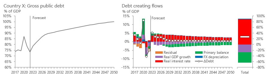
“Country X” benefits from having very low levels of foreign currency denominated debt, but does struggle to keep a sustainable path for its debt/GDP ratio given how high its real interest rate is. Measures to keep government accounts sustainable should target either to increase real GDP growth (via supply side reforms) or increasing its perceived structural primary balance (reducing spending or increasing tax collections). Otherwise debt/GDP will reach 100% by 2050.

Concluding thoughts

This is the second and final part of my series on fiscal analysis algebra. It covers four exercises that in my opinion widens our understanding about fiscal accounts. Most importantly, it brings economic concepts into how we analyse government balances and debt, shifting from the usual (and boring) accounting exercise. It also shows how a little algebra can take us a long way.

Thank you for making it this far, hope you enjoyed this one.