Applied linear algebra in economics - part 3

Shock identification and structural VARs

Welcome again. This is the 3rd post of a series where I explore vector autorregressions (VARs) as means to simulate and forecast economies. For context find links here (1st, 2nd). Today, I am going through what a structural vector autoregression (SVAR) model is and will try to better illustrate its purpose with an applied example.

As usual, I’m leaving an Excel spreadsheet linked somewhere in the text for those who want to study the exercise, I’ll leave it hidden in there to encourage the attentive reader.

Motivation

Before we dive straight into the math, I want to provide some motivation. In part 1, we stressed how one could simulate an economy using simple matrix representations as VAR models and briefly touched on “the identification challenge” that arises when working with real life data. Today’s post is about this very problem.

To illustrate this point, let’s just go straight to visualising the data. Below we present US GDP growth “y”, consumer price inflation excluding food and energy “π” and a constant maturity 3-month interest rate “i”.

We can note a visible contemporaneous positive relationship between the variables, when one goes up, so does the other. Growth rises and so does inflation rates, along with interest rates.

But wait, don’t central banks usually hike interest rates as a means to reduce inflation? Shouldn’t this be visible in the data?

This is what this motivation is about, the fact that dynamics matter and that economic theory needs to account for it properly before it can be applied to real life macroeconomics. If monetary policy committees can anticipate shifts and/or monitor the economy in real time, they are more prompt to steer policy rates in tandem with the economy. So if preliminary GDP indicators point to an increase in momentum which would later translate into higher inflation, they will hike policy rates today, not tomorrow. As a result, monetary policy rates and interest rates tend to be positively correlated to growth, because it is growth that tends to be the root cause of policy rate hikes, and markets anticipate that in short term bond yields too.

This makes the life of the applied macroeconomist slightly more challenging, as they are required to identify whether interest rates have been caused by growth expectations before they can assess the impact of a given monetary policy decision. This is the so called “identification problem”. Let’s bring some math into the analysis so we can explore this problem further.

Modelling

As you read in the first two posts of our Applied Linear Algebra series, a traditional way of analysing and forecasting economies is via vector autorregressions (VARs) estimated using least squares. The model can be presented as:

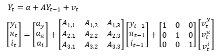
Here, “a’s” and “A’s” are parameters that we can estimate, and “v’s” are what we call model residuals. The least squares process is very straightforward: we isolate “v”, square both sides and minimise the squared “v” matrix (hence the name least squares” via an analytical optimisation technique.

If we analyse a shock in policy rates using impulse responses using this model, we get the underwhelming results below:

Results from impulse responses using a VAR(1) using data from 1985-2024

Puzzlingly, we see that after a policy rate hike, GDP growth increases but inflation falls. Is monetary policy so miraculously efficient that it can boost growth and kill inflation at the same time? Let’s hike interest rates to infinity then! Certainly these results are wrong, and they simply stem from the fact that our coefficient estimates are polluted by the positive contemporaneous relationships that arise due to the fact that economic agents have more than two brain cells and therefore can anticipate the future sometimes.

How can we make the model useful then? From simply reading the equation, we can note the problem that the model is specified so that contemporaneous variables are a function of past observations of eachother. We need to do better than that, and specify a model that allows for some contemporaneous responses alongside them. This is the Structural vector autorregression (SVAR). The pompous name simply stands for a vector autorregression that followed these algebraic steps:

Where the “A0” matrix is introduced to mediate how shocks are expected to affect our system contemporaneously. You will note that the resulting reduced form equation from the SVAR model is pretty much the same as the original VAR, only the parameter labels are changed. In matrix notation, this is how our new model looks like:

So the “A0” matrix introduced includes a parameter that shifts how monetary policy shocks “ε(i)” affect GDP growth “y” contemporaneously. This alone can change our policy rate shock analysis entirely. All we need to do is find a sensible number for the parameter “A0(i-y)”. Put simply, an SVAR model is simply a VAR whose residual “shock” matrices were constrained by theoretical stylised facts.

How do we come up with a number for “A0(i-y)” (and yes Elon feel free to use this to name your next child)? There are many ways, and I will only suggest one of them here. Given that the exercise is about “shock identification”, I thought it would be a good fit to use deviations from a policy rule to identify a monetary policy shock.

The argument for this approach goes as follows: central banks are expected to act, on average, in accordance to simple policy rules. When inflation exceeds the target or domestic demand overheats beyond its supply side capacity, they should hike interest rates accordingly, and vice-versa. This is the Taylor rule.

In the context of today’s post, it means that monetary policy shocks are loosely defined as any policy rate levels that can’t be explained by such rule. It means that the central bank stance is being discretionarily tighter/looser than what economic agents would expect given the rule. In equation form, it means the below:

Here, tilda accentuated variables denote deviations from target. “pi” is the inflation gap (minus target), and “y” is the output gap (GDP minus potential GDP). “i*” is the nominal neutral interest rate. Lastly, “c’s” are calibrated parameters.

As we draw a slope for how “ε(i)” is associated with “y”, we are able to identify a negative relationship within various sensible choices for the Taylor rule parameters. This allows us to use this exact slope as our “A0(i-y)” calibration.

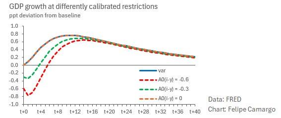
Plugging it in our SVAR model then produces the following impulse responses:

Which just so happens to be a much more sensible empirical result. Unsurprisingly, the impact of a policy rate shock to inflation is much more pronounced once we properly identify the impact of monetary policy in economic activity. Improved shock identification allowed us to see that much more clearly.

Under different (yet still sensible) Taylor rule calibrations, monetary policy shock estimates will result in slightly different interest rate slopes to growth, but responses remain consistent to theoretical expectations.

This simple “one-sheet” econometric exercise can be found in this link. Feel free to play with it as much as you want.

Concluding thoughts

Exercises that force us to think dynamically and bring economic theory to data improve the way we understand economics. In this post, we found that it is really hard to guess the impact of a policy decision without proper shock identification. This also happens to be a fundamental step into forecasting any economy.

For a more extensive theoretical exploration of shock identification in SVARs, this link is a very good starting point.

This is it for today’s entry, thank you for making it this far. If you enjoyed this post please don’t forget to like, subscribe and share it.