The unspoken truth about US fiscal policy

Who wants to be the one to rip off that bandaid?

Welcome. Today’s post aims to revisit some of the concepts discussed in previous posts and answer a relatively difficult question: What would be the cost to the global economy if the United States finally decided to pursue its much due fiscal adjustment?

Under conservative assumptions and reasonable methods, I find the cost to be about 1.3% of global GDP, excluding the cost to the US itself. To put it into perspective, this would amount to over US$ 900 bn in constant 2023 prices, which is approximately 1/4 of the cost paid to global output since the Covid-19 pandemic up to now. Yes, far from negligible numbers. No wonder policymakers avoid the subject.

How did I come up with these numbers? Allow me to walk you through it.

Debt sustainability algebra

The first step of our exercise is about identifying the exact size of the fiscal adjustment. In this post I’ve showed how to decompose public debt creating flows. We need to use our last equation, solving for the primary balance ‘pb*’ after assuming ‘Δd=0’. We’re supposed to yield:

\(pb_t^* = (\frac {r_t^w} {1+\delta_t})d_{t-1}+(\frac { \alpha_{t-1} [1+r_t^w]\epsilon_t} {1+\delta_t})d_{t-1}-(\frac {\delta_t} {1+\delta_t})d_{t-1} + \varepsilon_t\)

For the purposes of the US economy we can simplify this equation much further. US debt is mostly dollar denominated, and there seems to be no clear global world trend for the US dollar as a consensus, this makes ‘α’ and ‘ϵ’ parameters arguably small, very close to zero when multiplied by one another. We also can simplify the ‘ε’ as a white noise residual, bearing no importance on debt in the long run. Our final equation for the debt-stabilising primary balance is then reduced to:

\(pb_t^* = (\frac {r_t^w - \delta_t} {1+\delta_t})d_{t-1}\)

This equation states that the required primary balance to keep debt as a share of GDP constant depends on the difference between US gov’t weighted borrowing costs ‘r(w)’ minus GDP growth ‘δ’, discounted by one year of GDP growth and scaled back to debt/GDP levels.

Now its about coming up with assumptions for each of these variables.

I decided to anchor borrowing costs around current market yields, as does the CBO and other analysts, which are currently around 4.4% per year. If we consider a 2% annual average inflation target, this translates into ‘r(w)=2.4%’.

For growth, I’m using IMF’s assumption of 2% as a terminal rate, thus ‘δ=2%’.

The current US debt-to-GDP ratio is 123%, I’m sticking with this number.

Our debt-stabilising primary balance for the US economy is then 0.5%. If we take this years’ expectation for the primary deficit (around 3-3.5% of GDP), this would imply a 3.5-4ppts of GDP fiscal effort, that is, a reduction (increase) in primary spending (tax collections) to keep debt/GDP flat. This is how much the primary balance has to change, but there is more nuance to it, which I’ll explain in the next step.

The primary balance elasticity to fiscal spending

As explained previously in this other post, fiscal adjustments are not merely accounting exercises as they bear consequences to the rest of the economy.

When the government decides to tax more or spend less, households will consume and firms will invest less, affecting growth. This is very important as it translates into lower tax collections, making any fiscal adjustment much more costly than adding up public savings sources.

As a second step then, I try to account for some of that effect. We can assume a spending-based fiscal adjustment which would translate into a permanent loss in revenues and require a subsequent cut to spending until a new equilibrium is achieved where the primary fiscal balance parks at the required 0.5% of GDP primary surplus. This means we need to apply the following equation:

\(\frac {\Delta PB_t} {\Delta G_t} = \tau_t \kappa_t \epsilon^{Y \rightarrow T}_t -1\)

In this formula, the impact of a change in government spending to the primary balance is offset by its repercussions to tax collections, which depend on the tax burden ‘τ’, the fiscal multiplier ‘κ’ and the public revenue elasticity to GDP, ‘ϵ(Y→T)’.

As in the previous step, we now need to fill up each term of this equation with reasonable numbers. For the US economy, I’ve used 28% as the tax burden, 1.5 as the fiscal multiplier (a nice round number within public average estimates out there) and 1 as the revenue elasticity to GDP (just a rule of thumb, you do you). This means the primary balance is expected to change by a 0.58-to-1 change in primary spending ratio. Given that the required fiscal effort is of about 3.7ppts of GDP, we need an effective spending cut of 6.3ppts of GDP. This would end up hurting US output by 9.5% in the long run.

Massive isn’t it? This number has large caveats which could be better explored in different ways, as I’ll mention by the end of the post. For now lets keep it.

The third (and last) bit of this exercise is to link this to global-ExUS GDP. We’re almost there.

Vector autorregressions (VARs) and final results

There are many transmission mechanisms of US shocks to the global economy. Direct channels from trade, financial markets, or indirect, from confidence shocks to political repercussions and snowball effects on financial hurdles in fiscally distressed markets. For a blog post, I’d rather keep it simple and empirical.

To link US to global GDP here, I will resort to a very simple VAR(1) in annual frequency for an average response. In other previous posts, we have discussed in which contexts these can be estimated without issues regarding shock identifications. This would be a purely correlation-based association between what happened to the US on a given year and what followed on global GDP in the year after. The model is:

\(\begin{bmatrix} \Delta{y}^w_t \\ \Delta{y}^{us}_t \end{bmatrix} = \begin{bmatrix} a_0 \\ b_0 \end{bmatrix} + \begin{bmatrix} a_1 & a_2\\ b_1 & b_2 \end{bmatrix} \begin{bmatrix} \Delta{y}^w_{t-1} \\ \Delta{y}^{us}_{t-1} \end{bmatrix} + \begin{bmatrix} \varepsilon^w_{t} \\ \varepsilon^{us}_{t} \end{bmatrix}\)

Where ‘Δy(w)’ is the natural log change of global GDP excluding the US in constant 2015 bn dollars. ‘Δy(us)’ is the same, only for the US economy. ‘a’s and ‘b’s are parameters, and ‘ε’s shocks. It is a simple VAR indeed. I used annual data from 1960 to 2023 and got the following average coefficient estimates using least squares:

\(\begin{bmatrix} \Delta{y}^w_t \\ \Delta{y}^{us}_t \end{bmatrix} = \begin{bmatrix} 0.026 \\ 0.031 \end{bmatrix} + \begin{bmatrix} 0.168 & 0.111\\ -0.413 & 0.446 \end{bmatrix} \begin{bmatrix} \Delta{y}^w_{t-1} \\ \Delta{y}^{us}_{t-1} \end{bmatrix} + \begin{bmatrix} \varepsilon^w_{t} \\ \varepsilon^{us}_{t} \end{bmatrix}\)

Knowing that the US economy would correct against a baseline scenario without a fiscal adjustment by 9.5%, I’ve pencilled in a GDP correction in the US across 6 years through ‘ε(us)’ and computed the expected annual change to global growth and accumulated level GDP loss within twenty years to get the following chart.

VAR(1) impulse responses using World Bank GDP data

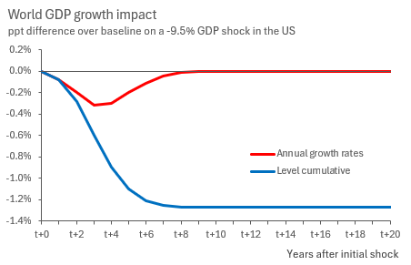
The cumulative level effect indicates a 1.3% permanent loss in global output. To put it into perspective, I have compared it against counterfactual post-pandemic losses, which indicates a loss of 5.2% level GDP against a 20-year trend. To compute a monetary loss, I re-scaled 1.3% cumulative losses to 2023 constant dollar GDP amounts using the US GDP deflator, which implies a US$ 912 bn loss to global output.

Log-linear trend sampled from 2000 to 2019 against observed data in the five subsequent years

Concluding thoughts

Today’s post was mostly my excuse to re-apply some of the tools that were previously discussed previously here as to come up with an answer to a reasonably difficult question.

There is certainly room for improvement in my calculations, for example putting way more effort into fully describing general equilibrium nuances to some of the estimates used (especially on the fiscal multiplier part). Yet I still believe there is value in this for most applied macroeconomists out there.

The post does not mean to imply a case against a fiscal adjustment in the US. In fact, it is a necessary evil that will worsen in time as is left unaddressed. The Monetary Fund is being very reasonable to recommend it sooner rather than later.

This is it for today. Thank you for making it this far.